All the code shown here is in this jupyter notebook

One of the problems that presented while implementing the lane lines detection project was translating a set of lines detected using the Hough method into a single line that we can draw into the screen, which represents the effective limits of the traffic lane. There were quite a number of questions surrounding the methods that can be used to extrapolate the Hough lines. This can be done in a number of ways, here I will present and explain some of them which I tested during the project.

Representing a line

The Hough transform returns a set of line segments which were detected from the image. These segments are represented by their start and end points, for example it will return an array in this shape:

[[[514, 326, 853, 538]], [[505, 324, 720, 464]]]

If we iterate the first dimension, each of the elements we get is a line. Then we can extract x1, y1, x2, y2 as the elements from the second dimension. This is a way to represent a line segment, but we know we can also represent the line that passes through this segment using the line equation:

 y = mx + b

Here, a given point in x will always have a corresponding coordinate in y, and this value will depend on the slope(m) of the line and the intercept(b), which is also the ‘y’ value when x = 0.

Once we have these two parameters we can draw any line segment we want(by fixing ‘x’ to the start and end points we want).

Now, another way to represent a line is by using a vector parallel to the line(so it has the same slope) and a point in the line. This describes the line completely because if you take such vector and translate it into the given point, you can get any segment of the line by multiplying this vector. To simplify things, the vector is usually normalized into a single unit length vector.

This should help picture what I mean, here the vector was already translated to the known point over the line:

Adjusting lines to sets of points

Now we know we have a set of lines given by the Hough transform, we can proceed to try to find a line that adjusts to this information.

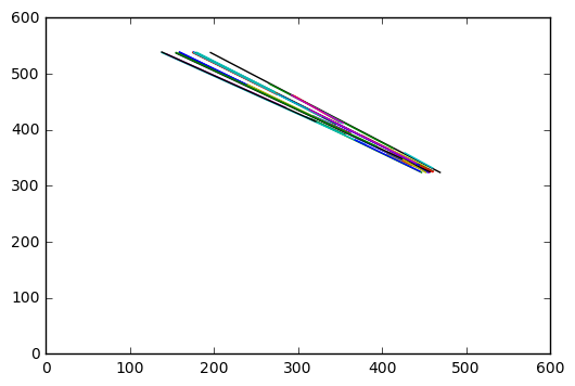
By drawing each one of the Hough lines, we get this plot:

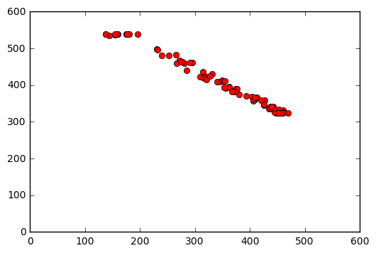
Another way of looking at this, is drawing each of the points given to us:

There are a couple basic ways to approach the problem of reducing this information to a single line:

• We can try adjusting a line that passes through this set of points while minimizing the total distance to each one of the points(method we call regression).
• We can also just average out the beginning points on one side, and the ending points on the other, and then, when we have these average points, adjust a line that passes through these.

The ‘fitline’ method

As stated, the first method we’re going to use is to try to fit a single line that minimizes the distance to all of the known points. To do this, we’re going to use the fitline() method from OpenCV. As you can see here, this method minimizes a distance function(which can be chosen using a parameter) to the given points. The result format is a four-element array, such as [vx,vy,x,y], where vx, vy are the unit vector coordinates and x, y are a point located in the line, as we discussed in the section above.

Applying this method to the points shown, we get these parameters:

vx [ 0.80845994]
vy [-0.58855116]
x [ 332.04876709]
y [ 417.42681885]

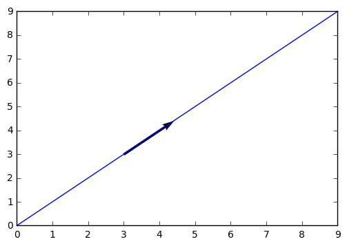
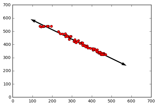
The normalized vector (vx, vy), translated to the coordinates origin looks like this:

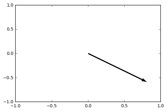
Once the vector is translated to the known point over the line, we can multiply it by either negative or positive values to get any vector over the lines(here we multiply by the same magnitude in both directions):

Now it’s easy get the slope and intercept parameters. We simply know that the slope of the line is equal to the one of the normalized vector, and we can use the known point to get the intercept value:

slope = vy / vx
intercept = y - (slope * x)

Which in this case turns out to be:

Slope [-0.72799051]
Intercept [ 659.15515137]

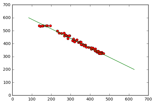
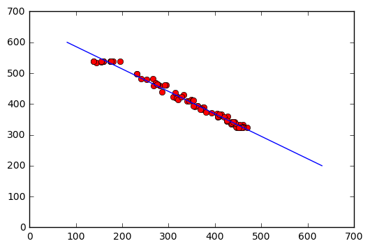
Given these two parameters, we can draw the line say from y=200 to y=600, simply:

startY = 200
endY = 600
startX = (startY - intercept) / slope
endX = (endY - intercept) / slope

And the resulting line:

Alternative method

The alternative method is a bit simpler to understand but it also seems to give good results, even when it is less sophisticated. What I did is run an average on the x, y coordinates first:

n = 1

for line in lines:
     for x1,y1,x2,y2 in line:
        x1Avg = x1Avg + (x1 - x1Avg)/n
        x2Avg = x2Avg + (x2 - x2Avg)/n
        y1Avg = y1Avg + (y1 - y1Avg)/n
        y2Avg = y2Avg + (y2 - y2Avg)/n
        n += 1

And then get the polynomial fit to the resulting average:

[slope, intercept] = np.polyfit([x1Avg, x2Avg], [y1Avg, y2Avg], 1)